Ejector CFD Simulation: Which Turbulence Model to Trust

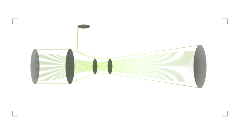
An ejector looks simple and is hard to simulate

An ejector has no moving parts and a handful of dimensions that matter. It ought to be easy to simulate. Then you run the same case with two turbulence models, and the entrainment ratio moves by more than the improvement you were hoping to design in.

Ejector CFD is unusually sensitive to modelling choices because the whole device works by turbulent mixing between a fast jet and a slow stream, usually with shocks in between. Here the turbulence model carries most of the physics. This article covers what a published validation study reports, which model to start with, and how to draw a conclusion you can defend from a result that carries an uncertainty of around 15%.

What is being predicted

The headline number is the entrainment ratio, the secondary mass flow divided by the primary mass flow. As an illustration, take a primary nozzle that passes 0.050 kg/s and an ejector that draws in 0.021 kg/s of secondary flow.

The second number is the critical back pressure, the highest outlet pressure at which the ejector still entrains at full capacity.

Three regimes, and why they matter for the simulation

An ejector behaves differently depending on its outlet pressure.

• Critical, or double-choked. Both the primary and the secondary flow are choked. The entrainment ratio is constant and does not respond to back pressure. This is the design regime and the kindest one to simulate, because choking fixes the mass flows almost independently of what happens downstream.
• Subcritical, or mixed. Above the critical back pressure the secondary flow is no longer choked, and the entrainment ratio falls steeply with every increment of outlet pressure. Small errors in the predicted mixing become large errors in the result.
• Malfunction. At still higher back pressure the primary flow backs up into the suction port.

Any conclusion from an ejector simulation should say which regime it applies to. A model that is good in the first can be useless in the second.

What a validation study reports

Besagni and co-authors at Politecnico di Milano compared several turbulence modelling approaches for supersonic ejectors against measurements. The k-ω SST model gave the best agreement. Its error in the entrainment ratio averaged 14%, with a maximum of 20%.

Those figures belong to the ejectors and conditions of that study, so read them as an order of magnitude. A carefully built model with k-ω SST can be expected within roughly 15% of the measured entrainment ratio in the design regime. In the subcritical regime, where the result is far more sensitive to the predicted mixing, expect less.

Why the model matters so much here

Three places in the flow decide the answer, and all three are hard for a two-equation model.

• The mixing layer. The primary jet drags the secondary stream along through a shear layer. How fast that layer spreads sets how much is entrained, and the spreading rate of compressible shear layers is something standard models are known to get wrong unless corrected.
• The shock train. Downstream of the nozzle, the flow adjusts to the local pressure through a series of shocks that interact with the boundary layer on the wall.
• The diffuser. The mixed stream has to recover pressure against an adverse gradient. Predict separation there too early or too late and the critical back pressure shifts.

k-ω SST was developed for adverse pressure gradients and separation, which is why it tends to do well here. The other two difficulties remain.

How I would set one up

• Start with k-ω SST and resolve the boundary layer on the mixing-section and diffuser walls. Wall functions are a poor match for the interaction between shocks and the boundary layer.
• Use an axisymmetric model for design conditions if the geometry allows. Go to three dimensions for off-design work or when the secondary inlet is clearly asymmetric.
• Use real fluid properties when the working fluid is steam or a refrigerant. Ideal-gas assumptions near saturation are a separate source of error, and for steam, condensation in the nozzle changes the picture again.
• Put the mesh where the mixing happens, at the nozzle exit, in the shear layer and in the constant-area section. Check mesh sensitivity on the entrainment ratio itself.
• Run a second turbulence model on the baseline. The gap between the two is a rough, honest indicator of model uncertainty for this particular ejector.
• Sweep the back pressure, even if only the design point interests you. You need to know how close to the critical point you are operating.

Drawing a conclusion from an uncertain number

Suppose the baseline gives an entrainment ratio of 0.42 and moving the nozzle exit 4 mm upstream gives 0.45. With a 15% uncertainty, the baseline alone could be anywhere between 0.36 and 0.48. Taken as two independent absolute values, the improvement is inside the noise.

The two runs share the mesh strategy, the turbulence model and its biases, so much of the error is common to both and cancels in the difference. The claim that moving the nozzle upstream raises the entrainment ratio by about 7% is far better supported than either absolute value.

That holds as long as both cases stay in the same regime. If the modified geometry sits closer to the critical point, the comparison crosses into territory where the model is weaker, and the conclusion needs a test.

In practice, validate one point if you possibly can, then use the model for trends around it.

Common mistakes

• Reporting an entrainment ratio without the regime. The number means little until the reader knows which side of the critical point it sits on.
• One mesh, one model, three significant figures. The precision of the printout says nothing about the accuracy of the model.
• Wall functions through the mixing section. The boundary layer there interacts with shocks and needs to be resolved.
• Ideal gas for steam near saturation. The property error adds to the turbulence-model error.
• Optimising a geometry at a single back pressure. The optimum can sit on the edge of the critical regime and collapse in service.

What a simulation is good for here

It will show you where the losses are, such as an over-expanded nozzle, a mixing section too short to finish mixing or a diffuser that separates. It will rank design changes reliably when they stay inside one regime, and it will tell you roughly where the critical back pressure lies.

A guaranteed entrainment ratio to two decimal places is beyond it. An ejector sold on a performance guarantee should have that guarantee confirmed on a rig.